Find change points efficiently in penalized linear regression models

fastcpd_lasso(data, ...)

fastcpd.lasso(data, ...)

# \donttest{
if (
  requireNamespace("ggplot2", quietly = TRUE) &&
    requireNamespace("mvtnorm", quietly = TRUE)
) {
  set.seed(1)
  n <- 480
  p_true <- 5
  p <- 50
  x <- mvtnorm::rmvnorm(n, rep(0, p), diag(p))
  theta_0 <- rbind(
    runif(p_true, -5, -2),
    runif(p_true, -3, 3),
    runif(p_true, 2, 5),
    runif(p_true, -5, 5)
  )
  theta_0 <- cbind(theta_0, matrix(0, ncol = p - p_true, nrow = 4))
  y <- c(
    x[1:80, ] %*% theta_0[1, ] + rnorm(80, 0, 1),
    x[81:200, ] %*% theta_0[2, ] + rnorm(120, 0, 1),
    x[201:320, ] %*% theta_0[3, ] + rnorm(120, 0, 1),
    x[321:n, ] %*% theta_0[4, ] + rnorm(160, 0, 1)
  )
  result <- fastcpd.lasso(
    cbind(y, x),
    multiple_epochs = function(segment_length) if (segment_length < 30) 1 else 0
  )
  summary(result)
  plot(result)

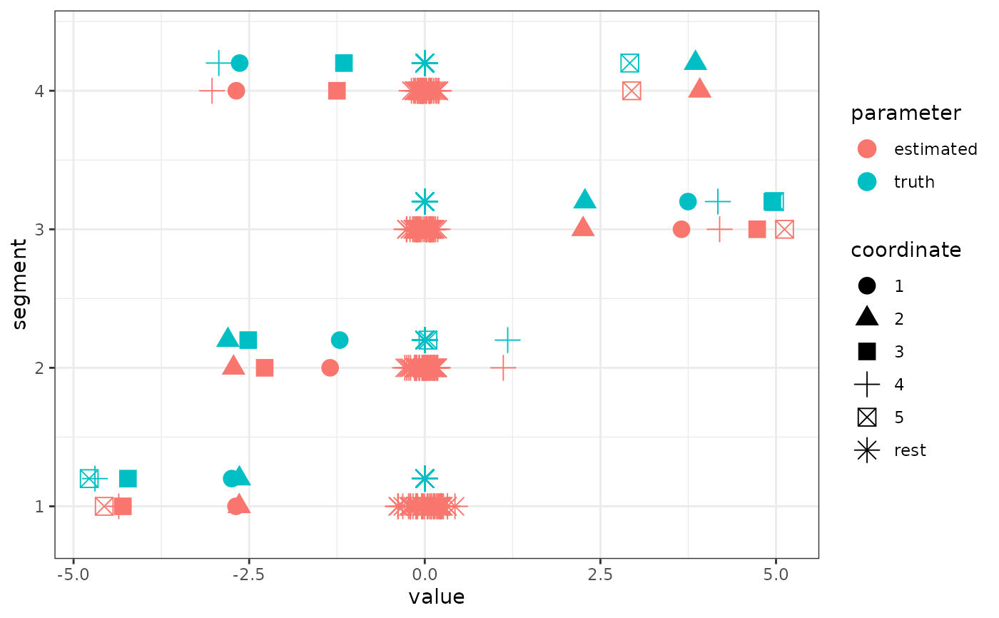
  # Combine estimated thetas with true parameters
  thetas <- result@thetas
  thetas <- cbind.data.frame(thetas, t(theta_0))
  names(thetas) <- c(
    "segment 1", "segment 2", "segment 3", "segment 4",
    "segment 1 truth", "segment 2 truth", "segment 3 truth", "segment 4 truth"
  )
  thetas$coordinate <- c(seq_len(p_true), rep("rest", p - p_true))

  # Melt the data frame using base R (i.e., convert from wide to long format)
  data_cols <- setdiff(names(thetas), "coordinate")
  molten <- data.frame(
    coordinate = rep(thetas$coordinate, times = length(data_cols)),
    variable = rep(data_cols, each = nrow(thetas)),
    value = as.vector(as.matrix(thetas[, data_cols]))
  )

  # Remove the "segment " and " truth" parts to extract the segment number
  molten$segment <- gsub("segment ", "", molten$variable)
  molten$segment <- gsub(" truth", "", molten$segment)

  # Compute height: the numeric value of the segment plus an offset for truth values
  molten$height <- as.numeric(gsub("segment.*", "", molten$segment)) +
    0.2 * as.numeric(grepl("truth", molten$variable))

  # Create a parameter indicator based on whether the variable corresponds to truth or estimation
  molten$parameter <- ifelse(grepl("truth", molten$variable), "truth", "estimated")

  p <- ggplot2::ggplot() +
    ggplot2::geom_point(
      data = molten,
      ggplot2::aes(
        x = value, y = height, shape = coordinate, color = parameter
      ),
      size = 4
    ) +
    ggplot2::ylim(0.8, 4.4) +
    ggplot2::ylab("segment") +
    ggplot2::theme_bw()
  print(p)
}
#> Warning: argument is not a function
#> 
#> Call:
#> fastcpd.lasso(data = cbind(y, x), multiple_epochs = function(segment_length) if (segment_length < 
#>     30) 1 else 0)
#> 
#> Change points:
#> 80 200 321 
#> 
#> Cost values:
#> 279.5634 294.3328 286.4413 318.8088 
#> 
#> Parameters:
#> 50 x 4 sparse Matrix of class "dgCMatrix"
#>       segment 1  segment 2 segment 3  segment 4
#>  [1,] -1.857418 -0.3996309  3.052401 -2.0014044
#>  [2,] -1.950296 -1.8422983  1.702204  3.3916313
#>  [3,] -3.260942 -1.6565430  4.201749 -0.5949362
#>  [4,] -3.807289  0.4543850  3.461070 -2.4616567
#>  [5,] -3.884467  .          4.390503  2.4178720
#>  [6,]  .         .          .         .        
#>  [7,]  .         .          .         .        
#>  [8,]  .         .          .         .        
#>  [9,]  .         .          .         .        
#> [10,]  .         .          .         .        
#> [11,]  .         .          .         .        
#> [12,]  .         .          .         .        
#> [13,]  .         .          .         .        
#> [14,]  .         .          .         .        
#> [15,]  .         .          .         .        
#> [16,]  .         .          .         .        
#> [17,]  .         .          .         .        
#> [18,]  .         .          .         .        
#> [19,]  .         .          .         .        
#> [20,]  .         .          .         .        
#> [21,]  .         .          .         .        
#> [22,]  .         .          .         .        
#> [23,]  .         .          .         .        
#> [24,]  .         .          .         .        
#> [25,]  .         .          .         .        
#> [26,]  .         .          .         .        
#> [27,]  .         .          .         .        
#> [28,]  .         .          .         .        
#> [29,]  .         .          .         .        
#> [30,]  .         .          .         .        
#> [31,]  .         .          .         .        
#> [32,]  .         .          .         .        
#> [33,]  .         .          .         .        
#> [34,]  .         .          .         .        
#> [35,]  .         .          .         .        
#> [36,]  .         .          .         .        
#> [37,]  .         .          .         .        
#> [38,]  .         .          .         .        
#> [39,]  .         .          .         .        
#> [40,]  .         .          .         .        
#> [41,]  .         .          .         .        
#> [42,]  .         .          .         .        
#> [43,]  .         .          .         .        
#> [44,]  .         .          .         .        
#> [45,]  .         .          .         .        
#> [46,]  .         .          .         .        
#> [47,]  .         .          .         .        
#> [48,]  .         .          .         .        
#> [49,]  .         .          .         .        
#> [50,]  .         .          .         .        


# }