Find change points efficiently in time series data

fastcpd_ts() and fastcpd.ts() are wrapper functions for fastcpd() to find change points in time series data. The function is similar to fastcpd() except that the data is a time series and the family is one of "ar", "var", "arma", "arima" or "garch".

Usage

fastcpd_ts(data, family = NULL, order = c(0, 0, 0), ...)

fastcpd.ts(data, family = NULL, order = c(0, 0, 0), ...)

Arguments

data

A numeric vector, a matrix, a data frame or a time series object.

family

A character string specifying the family of the time series. The value should be one of "ar", "var", "arima" or "garch".

order

A positive integer or a vector of length less than four specifying the order of the time series. Possible combinations with family are:

"ar", NUMERIC(1): AR(\(p\)) model using linear regression.
"var", NUMERIC(1): VAR(\(p\)) model using linear regression.
"arima", NUMERIC(3): ARIMA(\(p\), \(d\), \(q\)) model using stats::arima().
"garch", NUMERIC(2): GARCH(\(p\), \(q\)) model.

...

Other arguments passed to fastcpd(), for example, segment_count. One special argument can be passed here is include.mean, which is a logical value indicating whether the mean should be included in the model. The default value is TRUE.

Value

A fastcpd object.

Examples

# \donttest{
# Set seed for reproducibility
set.seed(1)

# 1. Define Parameters
n <- 500           # Total length of the time series
cp1 <- 200         # First change point at time 200
cp2 <- 350         # Second change point at time 350

# Define MA(2) coefficients for each segment ensuring invertibility
# MA coefficients affect invertibility; to ensure invertibility, the roots of
# the MA polynomial should lie outside the unit circle.

# Segment 1: Time 1 to cp1
theta1_1 <- 0.5
theta2_1 <- -0.3

# Segment 2: Time (cp1+1) to cp2
theta1_2 <- -0.4
theta2_2 <- 0.25

# Segment 3: Time (cp2+1) to n
theta1_3 <- 0.6
theta2_3 <- -0.35

# Function to check invertibility for MA(2)
is_invertible_ma2 <- function(theta1, theta2) {
  # The MA(2) polynomial is: 1 + theta1*z + theta2*z^2 = 0
  # Compute the roots of the polynomial
  roots <- polyroot(c(1, theta1, theta2))
  # Invertible if all roots lie outside the unit circle
  all(Mod(roots) > 1)
}

# Verify invertibility for each segment
stopifnot(is_invertible_ma2(theta1_1, theta2_1))
stopifnot(is_invertible_ma2(theta1_2, theta2_2))
stopifnot(is_invertible_ma2(theta1_3, theta2_3))

# 2. Simulate White Noise
e <- rnorm(n + 2, mean = 0, sd = 1)  # Extra terms to handle lag

# 3. Initialize the Time Series
y <- numeric(n + 2)  # Extra terms for initial lags (y[1], y[2] are zero)

# 4. Apply MA(2) Model with Change Points
for (t in 3:(n + 2)) {  # Start from 3 to have enough lags for MA(2)
  # Determine current segment
  current_time <- t - 2  # Adjust for the extra lags
  if (current_time <= cp1) {
    theta <- c(theta1_1, theta2_1)
  } else if (current_time <= cp2) {
    theta <- c(theta1_2, theta2_2)
  } else {
    theta <- c(theta1_3, theta2_3)
  }

  # Compute MA(2) value
  y[t] <- e[t] + theta[1] * e[t - 1] + theta[2] * e[t - 2]
}

# Remove the initial extra terms
y <- y[3:(n + 2)]
time <- 1:n

# Function to get roots data for plotting
get_roots_data <- function(theta1, theta2, segment) {
  roots <- polyroot(c(1, theta1, theta2))
  data.frame(
    Re = Re(roots),
    Im = Im(roots),
    Distance = Mod(roots),
    Segment = segment
  )
}

roots_segment1 <- get_roots_data(theta1_1, theta2_1, "Segment 1")
roots_segment2 <- get_roots_data(theta1_2, theta2_2, "Segment 2")
roots_segment3 <- get_roots_data(theta1_3, theta2_3, "Segment 3")

(roots_data <- rbind(roots_segment1, roots_segment2, roots_segment3))
#>          Re            Im Distance   Segment
#> 1 -1.173599 -5.752739e-16 1.173599 Segment 1
#> 2  2.840266  5.752739e-16 2.840266 Segment 1
#> 3  0.800000  1.833030e+00 2.000000 Segment 2
#> 4  0.800000 -1.833030e+00 2.000000 Segment 2
#> 5 -1.038071 -1.180701e-18 1.038071 Segment 3
#> 6  2.752357  1.180701e-18 2.752357 Segment 3

result <- fastcpd.ts(
  y,
  "arma",
  c(0, 2),
  lower = c(-2, -2, 1e-10),
  upper = c(2, 2, Inf),
  line_search = c(1, 0.1, 1e-2),
  trim = 0.04
)
summary(result)
#> 
#> Call:
#> fastcpd.ts(data = y, family = "arma", order = c(0, 2), lower = c(-2, 
#>     -2, 1e-10), upper = c(2, 2, Inf), line_search = c(1, 0.1, 
#>     0.01), trim = 0.04)
#> 
#> Change points:
#> 203 356 
#> 
#> Cost values:
#> 281.9365 227.2833 225.577 
#> 
#> Parameters:
#>    segment 1  segment 2  segment 3
#> 1  0.5078739 -0.4503097  0.6216729
#> 2 -0.3659708  0.2392382 -0.3661806
#> 3  0.8648758  1.0333590  1.1822530
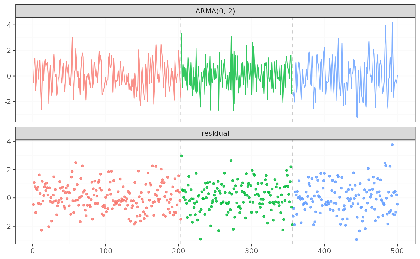
plot(result)

# }

Find change points efficiently in time series data

Usage

Arguments

Value

See also

Examples