Transcription Profiling of 57 Human Bladder Carcinoma Samples

Transcriptome analysis of 57 bladder carcinomas on Affymetrix HG-U95A and HG-U95Av2 microarrays

Usage

transcriptome

Format

A data frame with 2215 rows and 43 variables:

3: Individual 3
4: Individual 4
5: Individual 5
6: Individual 6
7: Individual 7
8: Individual 8
9: Individual 9
10: Individual 10
14: Individual 14
15: Individual 15
16: Individual 16
17: Individual 17
18: Individual 18
19: Individual 19
21: Individual 21
22: Individual 22
24: Individual 24
26: Individual 26
28: Individual 28
30: Individual 30
31: Individual 31
33: Individual 33
34: Individual 34
35: Individual 35
36: Individual 36
37: Individual 37
38: Individual 38
39: Individual 39
40: Individual 40
41: Individual 41
42: Individual 42
43: Individual 43
44: Individual 44
45: Individual 45
46: Individual 46
47: Individual 47
48: Individual 48
49: Individual 49
50: Individual 50
51: Individual 51
53: Individual 53
54: Individual 54
57: Individual 57

Source

<https://www.ebi.ac.uk/biostudies/arrayexpress/studies/E-TABM-147>

<https://github.com/cran/ecp/tree/master/data>

Examples

# \donttest{
if (requireNamespace("ggplot2", quietly = TRUE)) {
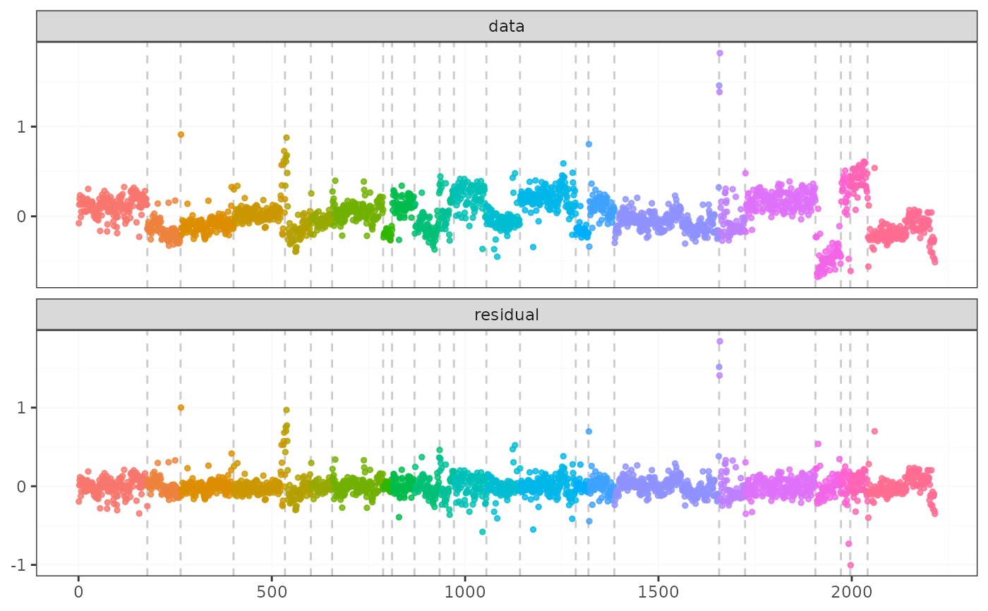
  result <- fastcpd.mean(transcriptome$"10", trim = 0.005)
  summary(result)
  plot(result)

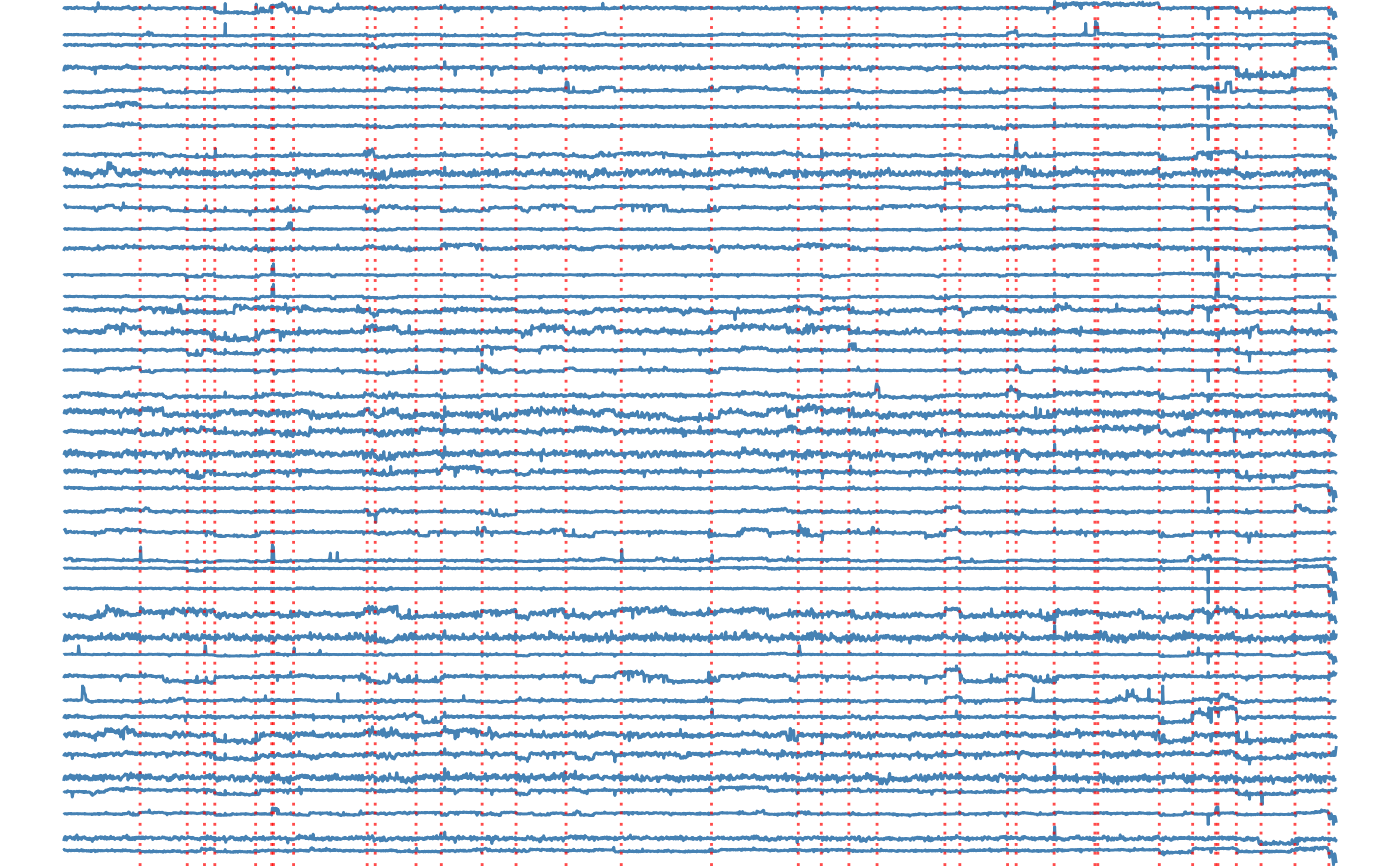
  result_all <- fastcpd.mean(
    transcriptome,
    beta = (ncol(transcriptome) + 1) * log(nrow(transcriptome)) / 2 * 5,
    trim = 0
  )

  plots <- lapply(
    seq_len(ncol(transcriptome)), function(i) {
      ggplot2::ggplot(
        data = data.frame(
          x = seq_along(transcriptome[, i]), y = transcriptome[, i]
        ),
        ggplot2::aes(x = x, y = y)
      ) +
        ggplot2::geom_line(color = "steelblue") +
        ggplot2::geom_vline(
          xintercept = result_all@cp_set,
          color = "red",
          linetype = "dotted",
          linewidth = 0.5,
          alpha = 0.7
        ) +
        ggplot2::theme_void()
    }
  )

  if (requireNamespace("gridExtra", quietly = TRUE)) {
    gridExtra::grid.arrange(grobs = plots, ncol = 1, nrow = ncol(transcriptome))
  }
}
#> 
#> Call:
#> fastcpd.mean(data = transcriptome$"10", trim = 0.005)
#> 
#> Change points:
#> 178 264 401 534 601 656 788 811 869 934 971 1055 1142 1286 1319 1386 1657 1724 1906 1972 1996 2041 
#> 
#> Cost values:
#> -312.3778 -152.8685 -223.128 -194.7351 28.05096 -110.2493 -234.4602 -48.13672 -104.2513 -95.29414 -34.57256 -118.7807 -135.2328 -228.7489 -66.44221 -93.27936 -388.8495 141.1922 -326.8845 -94.17653 -10.70687 -28.44282 -267.2412 


# }